Introduction to aramappings

Introduction to Adaptable Radial Axes (ARA) plots

Adaptable Radial Axes (ARA) plots (Rubio-Sánchez, Sanchez, and Lehmann 2017) are an interactive, exploratory data visualization technique related to Star Coordinates (Kandogan 2000, 2001) and Biplots (Gabriel 1971; Gower and Hand 1995; Hofmann 2004; Grange, Roux, and Gardner-Lubbe 2009; Greenacre 2010). ARA performs dimensionality reduction by representing high-dimensional numerical data as points in a plane or three-dimensional space. Unlike many other dimensionality reduction methods, ARA plots also visualize variable-specific information through “axis vectors” and their corresponding labeled axis lines, where each vector is associated with a particular data variable. These axis vectors (interactively defined by users, as in Star Coordinates) indicate the directions in which the values of their associated variables increase within the plot. Additionally, the high-dimensional observations are mapped (in an optimal sense) onto the plot in order to allow users to estimate variable values by visually projecting these points onto the labeled axes, as in Biplots.

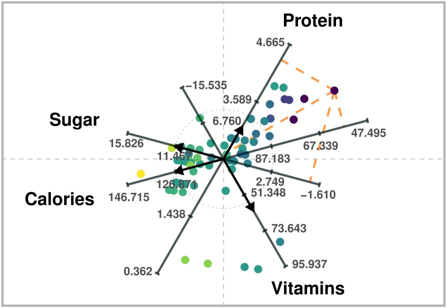
ARA plot of four variables of a breakfast cereal dataset. High-dimensional data values can be estimated via projections onto the labeled axes, as in Biplots.

In the previous ARA plot, the “axis” vectors associated with the variables are chosen to distinguish between healthier cereals (toward the right) and less healthy ones (toward the left). For instance, points on the right will generally have larger values of Protein and Vitamins, and lower values of Sugar and Calories. Users can obtain approximations of data values by visually projecting the plotted points onto the labeled axes. For example, users would estimate a value of about 57 calories for the point that lies further to the right.

Formal definition

ARA plots are obtained by solving the following general convex optimization problem:

\[\begin{array}{cl} \displaystyle \begin{array}{c}\mathrm{minimize} \\ \mathbf{P} \in \mathbb{R}^{N\times m} \end{array} & \hspace{-0.2cm} \begin{array}{c} \| (\mathbf{P}\mathbf{V}^{\scriptstyle \top} - \mathbf{X})\mathbf{W} \|, \\ \ \end{array} \\[10pt] \text{subject to} & \mathcal{C}. \\ \end{array}\]

Here, we use the following notation:

$N$: Number of data observations = number of mapped points.
$n$: Number of data variables.
$m$: Dimensionality of the visualization space (2 or 3).
$\mathbf{X}$: Data matrix of dimensions $N\times n$, where each row represents a data observation.
$\mathbf{V}$: $n\times m$ matrix of axis vectors. The $i$-th row is the axis vector associated with the $i$-th data variable.
$\mathbf{W}$: $n\times n$ diagonal matrix containing non-negative weights. The $i$-th weight is related to the $i$-th data variable.
$\mathbf{P}$: Matrix of mapped (or “embedded”) points of dimensions $N\times m$. Each row is the low-dimensional representation (i.e., the mapped point) of a data observation.
$\| \cdot \|$: A matrix norm.
$\mathcal{C}$: Some possible constraints.

Similarly to Biplots, the product $\mathbf{P}\mathbf{V}^{\scriptstyle \top}$ represents the estimates of data values in $\mathbf{X}$ when projecting the mapped points in $\mathbf{P}$ on to the axes defined by $\mathbf{V}$. Thus, the goal consists of finding optimal embedded points to minimize the discrepancy between the original data values and the estimates. Lastly, matrix $\mathbf{W}$ can be used to control relative accuracy of the estimates on each variable.

It is also worth noting that the variables should have a similar scaling. Otherwise, the solutions would focus on providing more accurate estimates for variables with larger values. In addition, centering the data leads to more accurate estimates in general. Thus, in practice, we recommend standardizing the data, which would center the data and force each variable to have unit variance.

Types of ARA plots

In the current version of the aramappings package there are 9 types of ARA plots, which stem from the combination of three types of matrix norms, and three choices regarding constraints.

Matrix norm

The current version of the package considers three norms:

$\| \cdot \|_{F}^{2}$: Squared $\ell^{2}$ (Frobenius) norm (sum of squares of the entries)
$\| \cdot \|_{1}$: $\ell^{1}$ norm (sum of absolute values of the entries)
$\| \cdot \|_{\infty}$: $\ell^{\infty}$ norm (maximum of absolute values of the entries)

The choice of norm reflects the analyst’s tolerance for large estimation errors. The $\ell^{\infty}$ norm emphasizes minimizing the maximum estimation error across all variables or axes, making it suitable when the worst-case error is critical. The $\ell^{2}$ norm also penalizes larger errors, but to a lesser extent. In contrast, the $\ell^{1}$ norm allows for some large estimation errors if doing so leads to significantly smaller errors for other variables.

Problem constraints

The current version of the package considers three options regarding the constraints of the ARA optimization problem:

Unconstrained problems. These formulations do not include constraints but may incorporate the weight matrix $\mathbf{W}$, which, in combination with the lengths of the axis vectors, can be used to control the desired relative accuracy when estimating values of specific variables. Variables with higher associated weights or longer axis vectors will receive greater emphasis in the optimization.
Exact estimates for one of the variables. In these problems, the weight matrix $\mathbf{W}$ is not used.
Ordered estimates for one variable. This variant imposes a weaker constraint. Instead of requiring exact value estimates for a variable, it is sufficient that the estimates preserve the ranking of the original data values. As with the exact case, the weight matrix $\mathbf{W}$ is not used in these formulations.

Available functions in aramappings

The aramappings package contains nine functions to compute ARA mappings (i.e., the embedded points in $\mathbf{P}$), according to the chosen norm and type of constraints. The names of thefunctions are shown in the following table:

	Unconstrained	Exact	Ordered
$\ell^{2}$ norm (squared)	`ara_unconstrained_l2()`	`ara_exact_l2()`	`ara_ordered_l2()`
$\ell^{1}$ norm	`ara_unconstrained_l1()`	`ara_exact_l1()`	`ara_ordered_l1()`
$\ell^{\infty}$ norm	`ara_unconstrained_linf()`	`ara_exact_linf()`	`ara_ordered_linf()`

The package also contains an additional basic function for drawing two-dimensional ARA plots when using standardized data:

draw_ara_plot_2d_standardized()

The function is included in order to show the results of the ARA mapping functions (i.e., the embedded points), together wirh the axis vectors and labeled axis lines. However, it does not consider several aspects that may be necessary for generating a clear visualization. Note that ARA should be implemented within an interactive visualization environment that offers extensive features. Such a tool should allow users to dynamically manipulate plots (e.g., by modifying axis vectors; customizing or toggling elements such as axes, labels, and variable names; encoding additional data dimensions through point color, size, or shape; and animating transitions between plots).

Installation

Install a stable version from CRAN

Install the development version of aramappings from GitHub with:

Usage examples

This section presents several usage examples.

Unconstrained ARA plot with the $\ell^{2}$ norm

We recommend starting an exploratory analysis using an unconstrained ARA plot with the $\ell^{2}$ norm, which can be generated very efficiently since the mappings ($\mathbf{P}$) can be obtained through a closed-form expression (i.e., a formula). The obvious first step is to load the aramappings package:

# Load package
library(aramappings)

In the usage examples we will use the Auto MPG dataset available in packages ascentTraining and grpnet, Kaggle, or the UCI Machine Learning Repository (Frank and Asuncion 2010). In this case, we load the dataset in the ascentTraining package.

# Load data
library(ascentTraining) # contains the Auto MPG dataset
data("auto_mpg")

Next, we select a subset of numerical variables from the dataset. The selected variables are specified through a vector containing their column indices in the original dataset. Furthermore, we rename the data set to X, simply for clarity with respect to the notation defined above.

# Define subset of (numerical) variables
selected_variables <- c(1, 4, 5, 6) # 1:"mpg", 4:"horsepower", 5:"weight", 6:"acceleration")

# Retain only selected variables and rename dataset as X
X <- auto_mpg[, selected_variables] # Select a subset of variables
rm(auto_mpg)

The ARA functions halt if the data or other parameters contain missing values. Thus, we proceed eliminating any row (data observation) that contains missing values. Naturally, another approach consists of replacing missing values by some other substituted values (imputation).

# Remove rows with missing values from X
N <- nrow(X)
rows_to_delete <- NULL
for (i in 1:N) {
  if (sum(is.na(X[i, ])) > 0) {
    rows_to_delete <- c(rows_to_delete, -i)
  }
}
X <- X[rows_to_delete, ]

At this moment X is a data.frame. In order to use the ARA functions we first need to convert it to a matrix:

# Convert X to matrix
X <- apply(as.matrix.noquote(X), 2, as.numeric)

In addition, we strongly recommend standardizing the data when using ARA. We save the result in variable Z since the function that draws the plot needs the original values in X.

# Standardize data
Z <- scale(X)

Having preprocessed the data, the next step consists of defining the axis vectors, which are the rows of $\mathbf{V}$. These can be obtained manually (ideally through a graphical user interface), or through an automatic method. For instante, $\mathbf{V}$ could be the matrix defining the Principal Component Analysis transfomation (in that case the ARA plot would be a Principal Component Biplot). In this example, we simply define a configuration of vectors in polar coordinates and transform them to Cartesian coordinates with the pol2cart() function in package geometry.

# Define axis vectors (2-dimensional in this example)
library(geometry)
r <- c(0.8, 1, 1.2, 1)
theta <- c(225, 100, 315, 80) * 2 * pi / 360
V <- pol2cart(theta, r)

It is also possible to define weights in order to control the relative importance of estimating accurately on each axis. This is nevertheless complex, since the accuracy also depends on the length of the axis vectors. In this case, we have set two weigths to 1 and another two to 0.75. Visually, the weights determine the level of gray used to color the axis vectors in the ARA plot.

# Define weights
weights <- c(1, 0.75, 0.75, 1)

Having defined the data (Z), axis vectors (V), and weights (weights), we can proceed to compute the ARA mapping. For unconstrained ARA plots with the $\ell^{2}$ norm the solver parameter should be set to “formula” (the default), in order to obtain the mapping through a closed-form expression. The following code computes the embedded points and saves them in mapping$P, and shows the execution runtime involved in computing the mapping.

# Compute the mapping and print the execution time
start <- Sys.time()
mapping <- ara_unconstrained_l2(
  Z,
  V,
  weights = weights,
  solver = "formula"
)
end <- Sys.time()
message(c('Execution time: ',end - start, ' seconds'))
#> Execution time: 0.00741314888000488 seconds

ARA plots can get cluttered when showing all of the axis lines and corresponding labels at the tick marks. Thus, the function that we will use to draw the ARA plot (draw_ara_plot_2d_standardized()) contains a parameter called axis_lines for specifying the subset of axis lines (and labels) we wish to visualize. In this example we will show the axes associated with variables “mpg” and “acceleration”. Note that in the original data frame these were variables 1 and 6. However, since we only retained four variables (“mpg”, “horsepower”, “weight”, and “acceleration”), the column index of “acceleration” is now 4.

# Select variables with labeled axis lines on ARA plot
axis_lines <- c(1, 4) # 1:"mpg", 4:"acceleration")

Also, the plotted points can be colored according to the values of a particular variable. In this example, we will color the points according to the value of variable “mpg”.

# Select variable used for coloring embedded points
color_variable <- 1 # "mpg"

Finally, we generate the ARA plot by calling draw_ara_plot_2d_standardized():

# Draw the ARA plot
draw_ara_plot_2d_standardized(
  Z,
  X,
  V,
  mapping$P,
  weights = weights,
  axis_lines = axis_lines,
  color_variable = color_variable
)
#> [1] 0

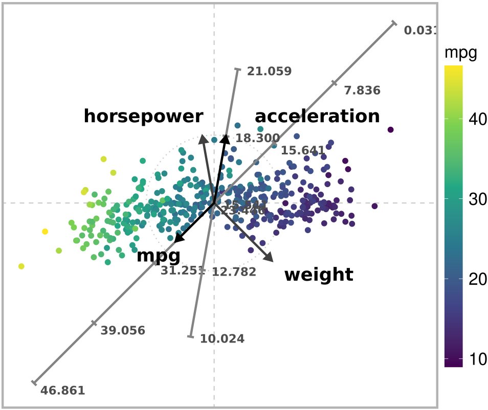
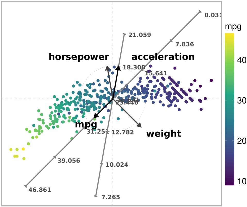
Unconstrained ARA plot with the l2 norm of a subset of the Autompg dataset.

Exact and ordered ARA plots

Exact and ordered ARA plots do not use weights, but it is necessary to specify the variable for which to obtain exact estimates, or for ordering the plotted points:

variable <- 1 # "mpg"

Exact ARA plot

The exact ARA mapping for the $\ell^{2}$ norm is computed through:

# Compute the mapping and print the execution time
start <- Sys.time()
mapping <- ara_exact_l2(
  Z,
  V,
  variable = variable,
  solver = "formula"
)
end <- Sys.time()
message(c('Execution time: ',end - start, ' seconds'))
#> Execution time: 0.713089466094971 seconds

Note that it is also very efficient since the solution can also be expressed as a formula. Finally, we generate the ARA plot:

# Draw the ARA plot
draw_ara_plot_2d_standardized(
  Z,
  X,
  V,
  mapping$P,
  axis_lines = axis_lines,
  color_variable = color_variable
)
#> [1] 0

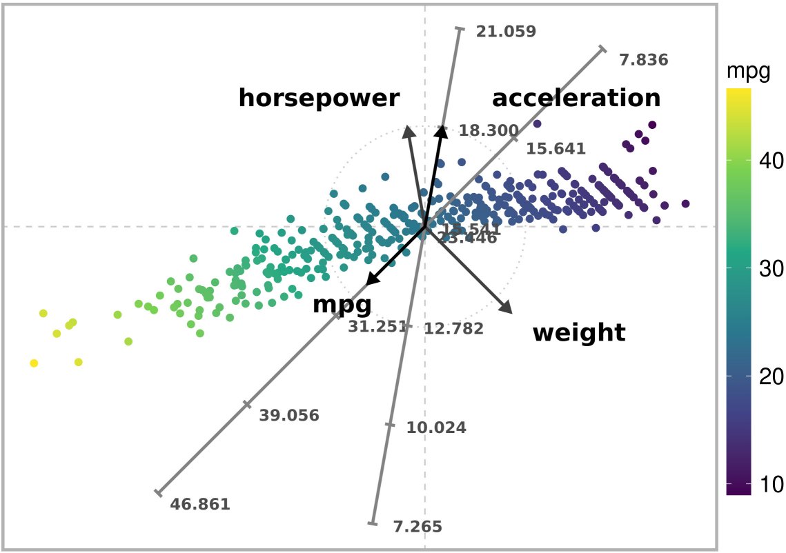
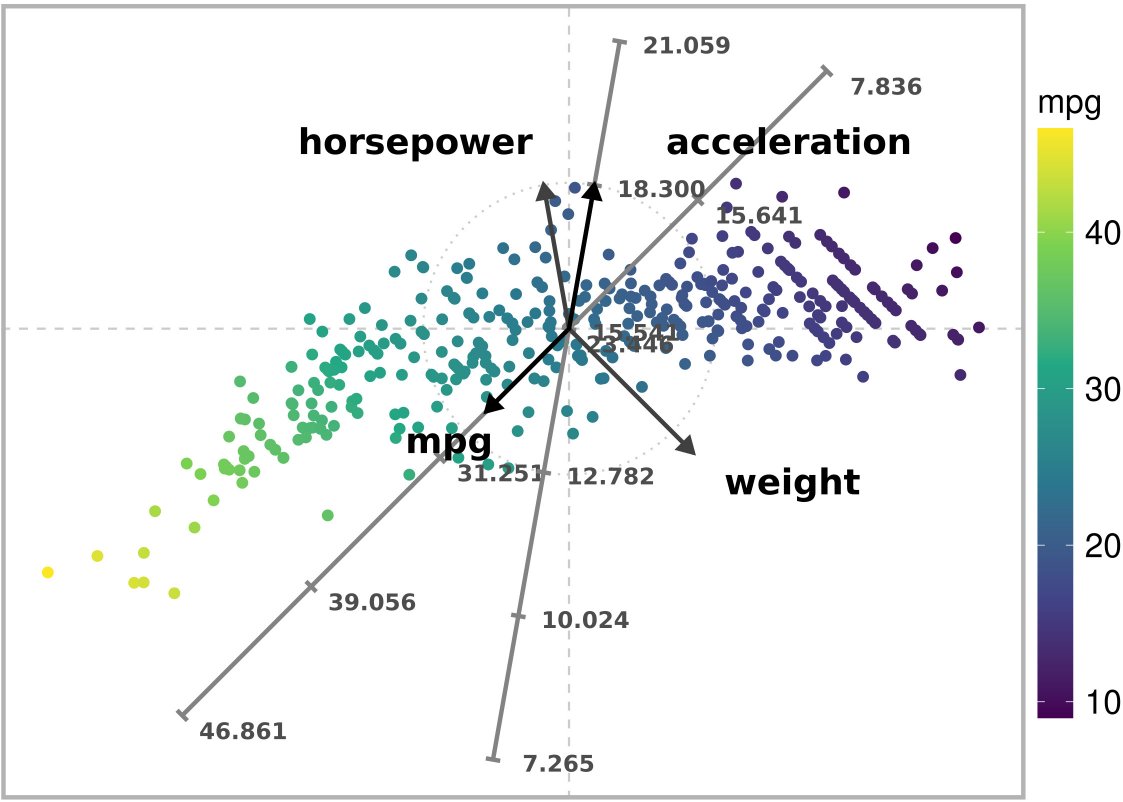
Exact ARA plot with the l2 norm of a subset of the Autompg dataset. Exact estimates are obtained for variable ‘mpg’.

Note that the colors of the plotted points are in consonance with their position along the “mpg” axis.

Ordered ARA plot

The optimization problem for the ordered ARA mapping with the $\ell^{2}$ is a quadratic program (QP). The following code solves the problem through the clarabel package.

# Compute the mapping and print the execution time
start <- Sys.time()
mapping <- ara_ordered_l2(
  Z,
  V,
  variable = variable,
  solver = "clarabel"
)
end <- Sys.time()
message(c('Execution time: ',end - start, ' seconds'))
#> Execution time: 0.0270786285400391 seconds

Finally, we generate the ARA plot:

# Draw the ARA plot
draw_ara_plot_2d_standardized(
  Z,
  X,
  V,
  mapping$P,
  axis_lines = axis_lines,
  color_variable = color_variable
)
#> [1] 0

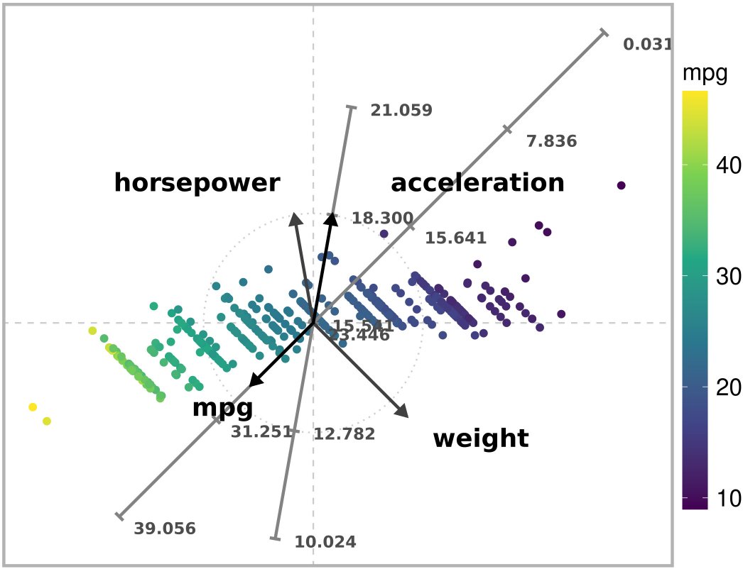
Ordered ARA plot with the l2 norm of a subset of the Autompg dataset. The values of ‘mpg’ are ordered correctly along its corresponding axis.

Although the estimates for “mpg” are not exact, the values of “mpg” are ordered correctly along the corresponding axes. In comparison with the exact mapping, the ordered variant produces more accurate estimates for other variables.

ARA plots using parallel processing

ARA mappings of unconstrained and exact problems with the $\ell^{1}$ or $\ell^{\infty}$ can be computed in parallel using several cores. The ideal number of cores to use depends on the size of the input data matrix. In general, it grows with the number of observations. Users are advised to analyze runtimes on their computers to estimate an adequate number of cores to use on their data.

In the following example, we first detect the available number of cores (NCORES) with package parallelly, and will use half of them (if several are available).

# Detect the number of available CPU cores
library(parallelly)
NCORES <- parallelly::availableCores()
if (NCORES > 1) {
  NCORES <- floor(NCORES / 2)
}

We then create a cluster object with function makeCluster() of the parallel package, specifying the number of cores to use.

# Create a cluster for parallel processing
cl <- parallel::makeCluster(NCORES)

In this example we will compute an ARA unconstrained mapping with the $\ell^{1}$ norm. This function admits weights, and lets us choose between several solvers. When using the solver from package glpkAPI we can specify whether to use a simplex algorithm, when parameter use_glpkAPI_simplex is set to TRUE, or an interior point method if it is set to FALSE. Lastly, the parameter cluster is the cluster object created above.

# Compute the mapping and print the execution time
start <- Sys.time()
mapping <- ara_unconstrained_l1(
  Z,
  V,
  weights = weights,
  solver = "glpkAPI",
  use_glpkAPI_simplex = TRUE,
  cluster = cl
)
end <- Sys.time()
message(c('Execution time: ',end - start, ' seconds'))
#> Execution time: 0.259163618087769 seconds

The ARA plot generated through:

draw_ara_plot_2d_standardized(
  Z,
  X,
  V,
  mapping$P,
  weights = weights,
  axis_lines = axis_lines,
  color_variable = color_variable
)
#> [1] 0

Unconstrained ARA plot with the l1 norm of a subset of the Autompg dataset.

Alternatively, the following code computes an exact ARA mapping with the $\ell^{1}$ norm:

# Compute the mapping and print the execution time
start <- Sys.time()
mapping <- ara_exact_l1(
  Z,
  V,
  variable = variable,
  solver = "glpkAPI",
  use_glpkAPI_simplex = TRUE,
  cluster = cl
)
end <- Sys.time()
message(c('Execution time: ',end - start, ' seconds'))
#> Execution time: 0.202067852020264 seconds

The ARA plot generated through:

draw_ara_plot_2d_standardized(
  Z,
  X,
  V,
  mapping$P,
  axis_lines = axis_lines,
  color_variable = color_variable
)
#> [1] 0

Exact ARA plot with the l1 norm of a subset of the Autompg dataset. Exact estimates are obtained for variable ‘mpg’.

Lastly, the cluster should be stopped at the end of the exploratory analysis process. It is not necessary to start a cluster and stop it after computing a single ARA mapping.

# Stop cluster
parallel::stopCluster(cl)

References

Frank, A., and A. Asuncion. 2010. “UCI Machine Learning Repository.” University of California, Irvine, School of Information; Computer Sciences. archive.ics.uci.edu/ml.

Gabriel, K. R. 1971. “The Biplot Graphic Display of Matrices with Application to Principal Component Analysis.” Biometrika 58 (3): 453–67. https://doi.org/10.1093/biomet/58.3.453.

Gower, John C., and David J. Hand. 1995. Biplots. Chapman & Hall/CRC Monographs on Statistics & Applied Probability. Taylor & Francis. https://doi.org/10.1002/(SICI)1097-0258(20000130)19:2<278::AID-SIM332>3.0.CO;2-3.

Grange, Anthony la, Niël le Roux, and Sugnet Gardner-Lubbe. 2009. “BiplotGUI: Interactive Biplots in r.” Journal of Statistical Software 30 (12): 1–37. https://doi.org/10.18637/jss.v030.i12.

Greenacre, Michael. 2010. Biplots in Practice. BBVA Foundation.

Hofmann, Heike. 2004. “COMPSTAT 2004 — Proceedings in Computational Statistics: 16th Symposium Held in Prague, Czech Republic, 2004.” In, 223–34. Heidelberg: Physica-Verlag HD. https://doi.org/10.1007/978-3-7908-2656-2_18.

Kandogan, Eser. 2000. “Star Coordinates: A Multi-Dimensional Visualization Technique with Uniform Treatment of Dimensions.” In Proceedings of the IEEE Information Visualization Symposium, Late Breaking Hot Topics, 9–12.

———. 2001. “Visualizing Multi-Dimensional Clusters, Trends, and Outliers Using Star Coordinates.” In Proceedings of the Seventh ACM SIGKDD International Conference on Knowledge Discovery and Data Mining, 107–16. KDD’01. New York, NY, USA: ACM. https://doi.org/10.1145/502512.502530.

Rubio-Sánchez, Manuel, Alberto Sanchez, and Dirk J. Lehmann. 2017. “Adaptable Radial Axes Plots for Improved Multivariate Data Visualization.” Computer Graphics Forum 36 (3): 389–99. https://doi.org/10.1111/cgf.13196.

	Unconstrained	Exact	Ordered
\(\ell^{2}\) norm (squared)	`ara_unconstrained_l2()`	`ara_exact_l2()`	`ara_ordered_l2()`
\(\ell^{1}\) norm	`ara_unconstrained_l1()`	`ara_exact_l1()`	`ara_ordered_l1()`
\(\ell^{\infty}\) norm	`ara_unconstrained_linf()`	`ara_exact_linf()`	`ara_ordered_linf()`