Draws a 2D Adaptable Radial Axes (ARA) plot for standardized data

Creates a plot associated with an Adaptable Radial Axes (ARA) mapping

Usage

draw_ara_plot_2d_standardized(
  Z,
  X,
  V,
  P,
  weights = rep(1, ncol(Z)),
  axis_lines = NULL,
  color_variable = NULL
)

Arguments

Z

Standardized numeric data matrix of dimensions N x n, where N is the number of observations, and n is the number of variables.

X

Original numeric data matrix (before standardizing) of dimensions N x n

V

Numeric matrix of "axis vectors" of dimensions n x 2, where each row of V defines an axis vector.

P

Numeric data matrix of dimensions N x 2 containing the N 2-dimensional representations of the data observations (i.e., the embedded points).

weights

Numeric array specifying non-negative weights associated with each variable. Can also be a 1D matrix. Default: array of n ones.

axis_lines

Array of integer variable indices (in [1,n]) indicating which calibrated axis lines are to be displayed. Default: NULL.

color_variable

Integer (in [1,n]) that indicates the variable used to color the embedded points. Default: NULL.

Value

Returns 0 if the function terminates without errors

Details

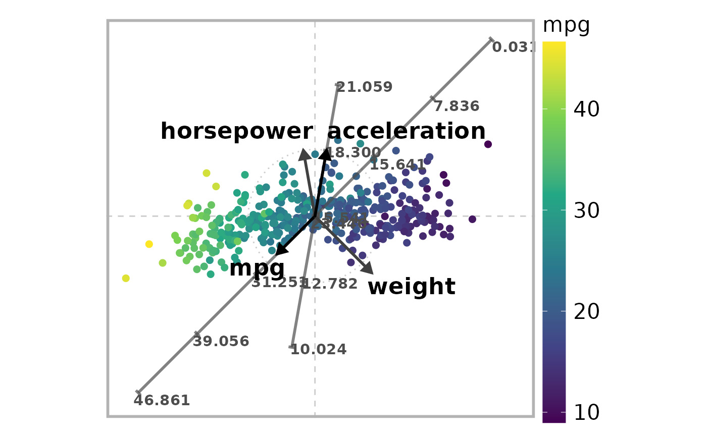
The function draw_ara_plot_2d_standardized() generates a basic two-dimensional plot related to an "Adaptable Radial Axes" (ARA) mapping (M. Rubio-Sánchez, A. Sanchez, and D. J. Lehmann (2017), doi: 10.1111/cgf.13196) for high-dimensional numerical data (X) that has been previously standardized (Z). The plot displays a set of 2D points (P), each representing an observation from the high-dimensional dataset. It also includes a collection of axis vectors (V), each corresponding to a specific data variable. If the ARA mapping incorporates weights (weights), these axis vectors are colored accordingly to reflect the weighting. For a user-specified subset of variables (axis_lines), the function additionally draws axis lines with tick marks that represent values of the selected variables. Users can estimate the values of the high-dimensional data by visually projecting the plotted points orthogonally onto these axes. The plotted points can also be colored according to the values of the variable color_variable.

References

M. Rubio-Sánchez, A. Sanchez, D. J. Lehmann: Adaptable radial axes plots for improved multivariate data visualization. Computer Graphics Forum 36, 3 (2017), 389–399. doi:10.1111/cgf.13196

Examples

# Load data
data("auto_mpg", package = "ascentTraining")

# Define subset of (numerical) variables
# 1:"mpg", 4:"horsepower", 5:"weight", 6:"acceleration"
selected_variables <- c(1, 4, 5, 6)

# Retain only selected variables and rename dataset as X
X <- auto_mpg[, selected_variables] # Select a subset of variables
rm(auto_mpg)
#> Warning: object 'auto_mpg' not found

# Remove rows with missing values from X
N <- nrow(X)
rows_to_delete <- NULL
for (i in 1:N) {
  if (sum(is.na(X[i, ])) > 0) {
    rows_to_delete <- c(rows_to_delete, -i)
  }
}
X <- X[rows_to_delete, ]

# Convert X to matrix
X <- apply(as.matrix.noquote(X), 2, as.numeric)

# Standardize data
Z <- scale(X)

# Define axis vectors (2-dimensional in this example)
r <- c(0.8, 1, 1.2, 1)
theta <- c(225, 100, 315, 80) * 2 * pi / 360
V <- geometry::pol2cart(theta, r)

# Define weights
weights <- c(1, 0.75, 0.75, 1)

# Compute the mapping
mapping <- ara_unconstrained_l2(Z, V, weights = weights, solver = "formula")

# Select variables with labeled axis lines on ARA plot
axis_lines <- c(1, 4) # 1:"mpg", 4:"acceleration")

# Select variable used for coloring embedded points
color_variable <- 1 # "mpg"

# Draw the ARA plot
draw_ara_plot_2d_standardized(
  Z,
  X,
  V,
  mapping$P,
  weights = weights,
  axis_lines = axis_lines,
  color_variable = color_variable
)
#> [1] 0