Unconstrained Adaptable Radial Axes (ARA) mappings using the L-infinity norm

ara_unconstrained_linf() computes unconstrained Adaptable Radial Axes (ARA) mappings for the L-infinity norm

Usage

ara_unconstrained_linf(
  X,
  V,
  weights = rep(1, ncol(X)),
  solver = "glpkAPI",
  use_glpkAPI_simplex = TRUE,
  cluster = NULL
)

Arguments

X: Numeric data matrix of dimensions N x n, where N is the number of observations, and n is the number of variables.
V: Numeric matrix defining the axes or "axis vectors". Its dimensions are n x m, where 1<=m<=3 is the dimension of the visualization space. Each row of V defines an axis vector.
weights: Numeric array specifying optional non-negative weights associated with each variable. The function only considers them if they do not share the same value. Default: array of n ones.
solver: String indicating a package for solving the linear problem(s). It can be "clarabel" (default), "glpkAPI", "Rglpk", or "CVXR".
use_glpkAPI_simplex: Boolean parameter that indicates whether to use the simplex algorithm (if TRUE) or an interior point method (if FALSE), when using the glpkAPI solver. The default is TRUE.
cluster: Optional cluster object related to the parallel package. If supplied, and n_LP_problems is N, the method computes the mappings using parallel processing.

Value

A list with the three following entries:

P: A numeric N x m matrix containing the mapped points. Each row is the low-dimensional representation of a data observation in X.
status: A vector of length N where the i-th element contains the status of the chosen solver when calculating the mapping of the i-th data observation. The type of the elements depends on the particular chosen solver.
objval: The numeric objective value associated with the solution to the optimization problem, considering matrix norms, and ignoring weights.

If the chosen solver fails to map one or more data observations (i.e., fails to solve the related optimization problems), their rows in P will contain NA (not available) values. In that case, objval will also be NA.

Details

ara_unconstrained_linf() computes low-dimensional point representations of high-dimensional numerical data (X) according to the data visualization method "Adaptable Radial Axes" (M. Rubio-Sánchez, A. Sanchez, and D. J. Lehmann (2017), doi: 10.1111/cgf.13196), which describes a collection of convex norm optimization problems aimed at minimizing estimates of original values in X through dot products of the mapped points with the axis vectors (rows of V). This particular function solves the unconstrained optimization problem in Eq. (10), for the L-infinity vector norm. Specifically, it solves equivalent linear problems as described in (12). Optional non-negative weights (weights) associated with each data variable can be supplied to solve the problem in Eq. (15).

References

M. Rubio-Sánchez, A. Sanchez, D. J. Lehmann: Adaptable radial axes plots for improved multivariate data visualization. Computer Graphics Forum 36, 3 (2017), 389–399. doi:10.1111/cgf.13196

Examples

# Load data
data("auto_mpg", package = "ascentTraining")

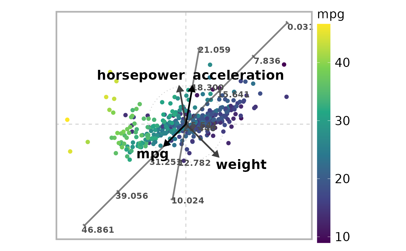
# Define subset of (numerical) variables
# 1:"mpg", 4:"horsepower", 5:"weight", 6:"acceleration"
selected_variables <- c(1, 4, 5, 6)

# Retain only selected variables and rename dataset as X
X <- auto_mpg[, selected_variables] # Select a subset of variables
rm(auto_mpg)
#> Warning: object 'auto_mpg' not found

# Remove rows with missing values from X
N <- nrow(X)
rows_to_delete <- NULL
for (i in 1:N) {
  if (sum(is.na(X[i, ])) > 0) {
    rows_to_delete <- c(rows_to_delete, -i)
  }
}
X <- X[rows_to_delete, ]

# Convert X to matrix
X <- apply(as.matrix.noquote(X), 2, as.numeric)

# Standardize data
Z <- scale(X)

# Define axis vectors (2-dimensional in this example)
r <- c(0.8, 1, 1.2, 1)
theta <- c(225, 100, 315, 80) * 2 * pi / 360
V <- geometry::pol2cart(theta, r)

# Define weights
weights <- c(1, 0.75, 0.75, 1)

# Detect the number of available CPU cores
NCORES <- parallelly::availableCores(omit = 1)

# Create a cluster for parallel processing
cl <- parallel::makeCluster(NCORES)

# Compute the mapping
mapping <- ara_unconstrained_linf(
  Z,
  V,
  weights = weights,
  solver = "glpkAPI",
  use_glpkAPI_simplex = TRUE,
  cluster = cl
)

# Stop cluster
parallel::stopCluster(cl)

# Select variables with labeled axis lines on ARA plot
axis_lines <- c(1, 4) # 1:"mpg", 4:"acceleration")

# Select variable used for coloring embedded points
color_variable <- 1 # "mpg"

# Draw the ARA plot
draw_ara_plot_2d_standardized(
  Z,
  X,
  V,
  mapping$P,
  weights = weights,
  axis_lines = axis_lines,
  color_variable = color_variable
)
#> [1] 0